Cover photo by Waldemar Brandt on Unsplash. In Italy, when someone is speaking nonsense or is saying something outrageously wrong, we say that he’s “giving away the numbers”. Hopefully we’ll be able to retain our mental fitness and say a lot of very correct stuff, while still giving away some numbers in a literal sense.

What you should know before reading this post

• Basic linear algebra
• Basic calculus

The quest for numerical integration

There comes a point where our nice theoretical results, with closed formulas and all that jazz, are no longer sufficient to make a decision, give an estimate or complete our task. Sometimes we just need a number, a nicely written one using only digits, commas and some scientific notation for the adventurous. A particular class of problems that arises in obtaining our dear number is the one of numerical integration. Riemann and Lebesgue integrals are not particularly wieldy objects to begin with (that’s the reason why they’re plenty of fun, no?) and Ito integrals are even worse. In fact, for Ito intergrals, it’s quite hard to even state what a solution written with just digits is. Do we want a path-wise solution or do we just need some statistical properties to hold? We will try to get a grasp of all this tough stuff. But every nice journey begins with, well… the beginning. This is part of a series of 3 articles:

• 🙋‍♂️ Numerical (algebraic) interpolation, the basis for numerical integration;
• Numerical approximation of Riemann integrals;
• Numerical approximation of Ito integrals, specifically targeting the issue of finding a weakly converging approximation scheme for processes built on the browninan motion (spoiler: this is what we need to price our beloved financial products).

This time we are going to face the task of algebraic interpolation. While this article is going to be pretty far from being exhaustive (to be honest, there are 300 pages long books about interpolation which are pretty far from being exhaustive), it will serve as a starting point for our journey and I hope it will stimulate your curiosity. Well, enough preambles: 1, 2, 3, take a deep breath and… let’s get going!

What even is interpolation?

The problem of interpolation arises when we want to find a function \(f(x)\) such that given a point cloud \((x_{i},y_{i})_{i = 1, 2, 3, \dots}\) we have \(f(x_{i})=y_{i}\). In particular, algebraic interpolation is the issue of finding \(f\) among the family of polynomials or piecewise polynomial functions. When the function is only piecewise polynomial, we are talking about spline interpolation. A case of particular interest is when there exists a known function \(\varphi(x)\) such that \(y = \varphi(x)\), where \(\varphi(x)\) has some unpleasant properties that make it difficult to evaluate. Another scenario where interpolation is useful is when \(\varphi(x)\) has some known properties but doesn’t allow for an explicit closed form. In this case we may still want to use a polynomial to approximate \(\varphi\), since polynomials are easy to handle and evaluate. There will be errors in doing this: we are going to measure them using the \(\infty\)-norm.

Definition. (Approximation error)

Given an interval \(I \subset \mathbb{R}\) and a function \(\varphi: I \to \mathbb{R}\) we define the approximation error obtained approximating \(\varphi\) over \(I\) using a polynomial \(f\), \(E(f;\varphi)_{I}\) as

\begin{equation} E_{I}(f; \varphi) = \| f - \varphi \| _{ \infty } \restriction _{I} \end{equation}

∎

This is our first glimpse of the essential nature of numerical analysis: knowing that you are wrong and by how much is even more important than the number you get at the end. Just as a note, sometimes you may mitigate this limitation of numerical analysis using tools like symbolic machine algebra. In theory, we can be quite successful at approximating functions by polynomials, we just need our functions to be continuous:

Theorem. (Weierstrass Theorem on approximation errors)

Let \(\varphi\) be a continuous function on some interval \(I\). Then for any \(\varepsilon > 0\) there exists \(n \in \mathbb{N}\) and a polynomial \(P_n\) of degree \(n\) such that \(E_{I}(P_n; \varphi) < \varepsilon\)

∎

J-L. Lagrange in 1795 had the brilliant idea to define a vector space of polynomials with degree equal to the number of points in the cloud minus one. Lagrange polynomials have the nice property of having unit value on the various \(x_{i}\), and they constitute a basis for the linear space of polynomials, so that the interpolating polynomial is just a vector whose components are the \(y_{i}\). They look as follows:

Definition. (Lagrange polynomials)

Given a point cloud \((x_{i},y_{i})_{i = 1, 2, 3, \dots, n}\) we define the Lagrange basis of the \(n\)-degree polynomials space as

\begin{equation} l_{k}=\frac{\pi_{n}(x)}{\pi_{n}’(x) (x-x_{k})} \end{equation}

where \(\pi_{n}=(x-x_{1})(x-x_{2}) \dots (x-x_{n})\).

∎

Evaluating the Lagrange interpolating polynomial \(L_{n}=y_{1}l_{1} + \dots + y_{n}l_{n}\) has computational complexity \(\mathcal{O}(n^{2})\), which is quite nice. Anything polynomial is actually nice, NP-hard problems are a massive issue.

Where should I put my \(x_{i}\)?

Choosing where to evaluate the “hard” function before approximation plays a massive role in how good our interpolation will be. In fact we have this theorem:

Theorem. (First Faber’s theorem)

For any a priori known algorithm for determining the \(x_{i}\) independently of the target function \(\varphi\), there exist both a target function such that the approximation error does not converge to \(0\) as the number of \(x_{i}\) increases and one such that the approximation does indeed converge to \(0\) as \(n\) goes to infinity.

∎

So, no matter how smart we are in pre-determining the \(x_{i}\) (from here on called nodes), sometimes we get things terribly wrong. But we can still be pretty smart. The following theorem tells us that we can bound the error by means of a recursive relation:

Theorem. (Lebesgue constants theorem)

Let \(\varphi\) be a continuous target function on some interval \(I\). Then the following relation holds

\begin{equation} E_{I}(L_{n}; \varphi) \leq (1+\Lambda_{n}((x_{i})_{i = 1, \dots, n})) \mathcal{E}_{n-1}(\varphi) \end{equation}

where \(\Lambda_{n} = \| \lambda_{n} \| _{\infty} \restriction_{I}\) are called Lebesgue’s constants, the \(n\)-th Lebesgue function \(\lambda_{n}\) is the sum of the absolute values of the Lagrange basis polynomials and \(\mathcal{E}(\varphi)\) is the best possible polynomial approximation of \(\varphi\) using polynomials of degree \(n\).

∎

Given the recursive nature of this error bound, we would like to find an algorithm for selecting the nodes that allows us to have the Lebesgue constants grow as slowly as possible as we increase the number of nodes. There is, however, a limit to how slowly we can have them grow.

Theorem. (Second Faber’s theorem)

For any choice of node system, we have \(\Lambda_{n}((x_{i})_{i = 1, \dots, n}) \geq \frac{1}{12} \log (n)\)

∎

Therefore, we have that if Lebesgue constants grow logarithmically, the node system has optimal scaling. Unsurprisingly, the smoothness of the target function also plays an important role.

Theorem

Let \(\varphi\) be a \(k\)-times differentiable target function on some interval \(I\). Then the following relation holds

\begin{equation} E_{I}(L_{n}; \varphi) \leq c \frac{\log n}{n^k} \end{equation}

where \(c\) is independent of \(k\) and \(n\)

∎

This is it for the general facts. Let’s have a small recap befor moving on:

• interpolating basically means joining points in a nice way. And polynomials are really nice;
• Weierstrass’ theorem makes it looks like algebraic interpolation can in theory be infinitely effective;
• Lagrange gave us a way of choosing the coefficients for our interpolating polynomial that just works;
• we can estimate errors;
• Faber’s theorems shattered our dreams of a universally good way of picking the interpolation nodes.

Our main focus is the choice of the node system, let’s see some of those and let’s try to say something about their performance.

Some notable node systems

The first thing we would like to do is to use evenly spaced nodes across our interval. This seemingly reasonable choice is, unfortunately, an awful one.

Theorem. (Tureckij theorem)

For an evenly spaced system of nodes the Lebesgue constants have the following scaling:

\begin{equation} \Lambda _ {n} ((x_{i})_{i = 1, \dots, n})) \sim \frac{2^{n}}{e n \log n} \end{equation}

∎

This is related to an unpleasant phenomenon that we are going to see later, called the Runge effect. This leads many practitioners to limit the usage of evenly spaced nodes only with polynomials of degree at most equal to nine. We have smarter choices available, but first we need some extra notions.

Definition. (Orthogonal polynomials)

Two degree \(n\) polynomials \(p\) and \(q\) defined on the interval \([-1,1]\) are said to be orthogonal with respect to the \(\alpha , \beta\)-Jacobi weighted inner product if they satisfy the following condition

\begin{equation} \int_{-1}^{1} p(x) q(x) (1-x)^{\alpha}(1+x)^{\beta} dx = 0 \end{equation}

∎

Note that we can always traslate our approximation problem from a generic bounded interval into \([-1,1]\) by means of an affine transform. The roots of the orthogonal polynomial defined as before have several nice properties. We will refer to the node system given by these roots as \(w^{\alpha , \beta}\).

Theorem. (Szegő theorem)

If \(\alpha\) and \(\beta\) belong in \((-1,\frac{1}{2}]\), then the scaling of the Lebesgue constants of \(w^{\alpha , \beta}\) is logarithmic, and it is polynomial otherwise.

∎

Szegő theorem therefore states how to reach that optimal logarithmic scaling of the error bound we were looking for. Sometimes, a process called enrichment is needed even when we are within the conditions stated by the theorem. We won’t talk about this process, but it basically is a way of adding nodes to improve performance. We will perform practical tests on two system of nodes of particular importance: the evenly spaced nodes (that we will indicate with \(\mathcal{E}\) ) and the the roots of the Chebyshev polynomials of the first kind ( \(P_{n} = \cos (n \arccos \theta)\) ), which is \(w^{- \frac{1}{2} , -\frac{1}{2}}\). When using \(w^{- \frac{1}{2} , - \frac{1}{2}}\), it can be proved that for differentiable target functions the approximation error is guaranteed to converge to zero. I encourage you to research \(w^{0 , 0}\), which are the roots of the Legendre polynomials and \(w^{\frac{1}{2} , \frac{1}{2}}\) which are the roots of the Chebyshev polynomials of the second kind. These two node system need enrichment to work optimally. It’s quite remarkable how Jacobi weights can describe a family of polynomials that contains so many notable specimens.

Node systems, tested

First of all we need to evaluate the roots of the Chebyshev polynomials: playing around with the definition will show that our roots are given by \(x_{i}=cos(\frac{\pi (i+\frac{1}{2})}{n})\) as \(i\) spans over \(0, \dots, n-1\). This is implemented in chebyshevPolynomialRoots.m:

          function xNodes = chebyshevPolynomialRoots( degree, targetIntervalLowerBound, targetIntervalUpperBound )
            xRaw = zeros( degree, 1 );    
            for i = 0 : degree - 1 
                    xRaw( i + 1 ) = cos( pi * ( i + 0.5) / degree );
            end
            xRaw = sort( xRaw );
            xNodes = 0.5 * xRaw ...
                        * ( targetIntervalUpperBound - targetIntervalLowerBound ) ...
                        + mean( [ targetIntervalLowerBound targetIntervalUpperBound ] );
          end

Now we need a routine to evaluate our interpolating polynomial. Here it is, lagrangePoly.m:

          function y = lagrangePoly( nodes, components, x )
              piCoeff = poly( nodes );
              dPiCoeff = polyder( piCoeff );
              y = zeros( 1, length( x ) );
              for i = 1 : length( components )
                    y = y + ...
                        components(i) * ...
                        polyval( piCoeff, x ) ./ ...
                        ( polyval( dPiCoeff, nodes( i ) ) .* ( x - nodes( i ) ) );
              end
          end

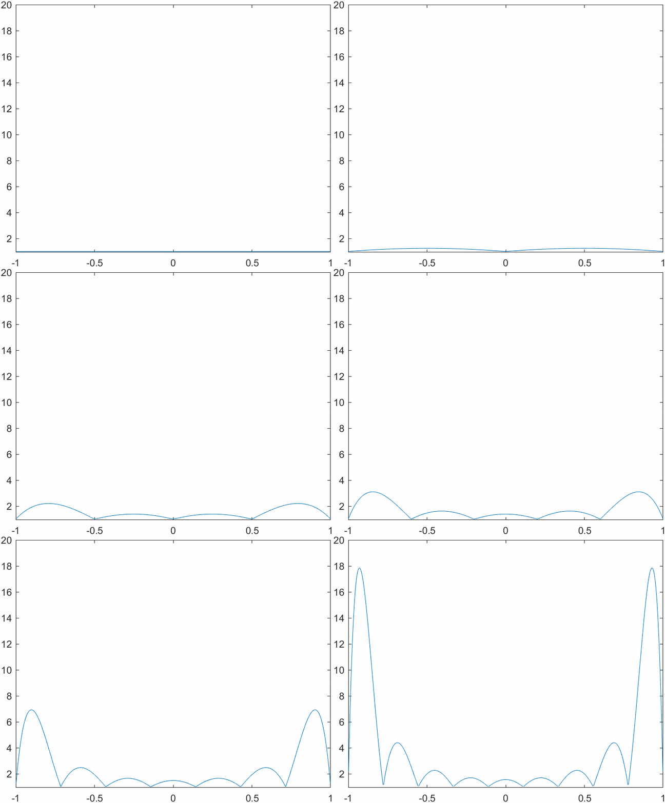
This code allows us to evaluate the Lebesgue functions for different combinations of number of nodes and nodes system. First of all we will analyze the behavior of the Lebesgue functions in a system with evenly spaced nodes: note how the magnitude explodes near the edges of the interpolation interval. This is tightly related to the Runge phenomenon. Think about the definition of the Lebesgue functions: why is their value \(1\) on the nodes?

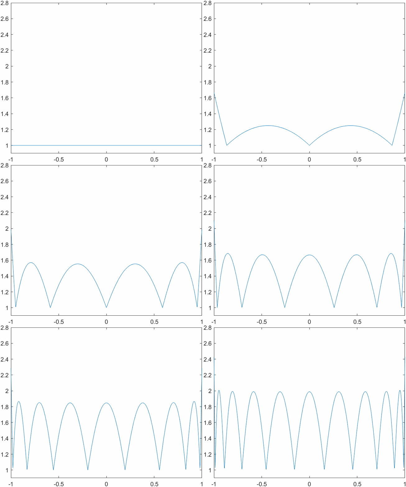
This is how things change when we switch to the Chebyshev node system. The magnitude of the functions varies more evenly across the interval, yielding a better bound for the interpolation error.

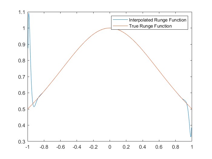
Lastly, we take a look at the Runge phenomenon. When approximating \(\frac{1}{1+x^2}\) using algebraic interpolation on a system of 32 evenly spaced nodes we can see instabilities on the edges of the interval. This is related to the behavior of the Lebesgue functions that we saw in a previous figure. If we were to use the Chebyshev node system, the plot of the interpolated approximation and the one of the true function would be pretty much identical.

What about splines?

Splines can be more advantageous as they usually yield good results even when using very simple interpolating functions. Some of the most common splines that are used in practical applications are linear and cubic splines (when dealing with functions from \(\mathbb{R}\) to \(\mathbb{R}\) ) and Beziér splines (when dealing with curves in a space or in a plane). Usually one will find that the approximation error with splines is a function of the distance between the nodes \(h\). Consider this example: how can we bound the spline approximation error for a twice differentiable function over a system of evenly spaced nodes? Let \(x_{i}\) and \(x_{i+1}\) be two consecutive nodes, and let \(x\) be a point in between these two nodes. Let \(s(x)=a_{s}x+b_{s}\) be the restriction of the spline to the interval \([ x_{i}, x_{i+1} ]\). Let \(q\) be a constant, independent of \(x\). Define the function \(g(y)\) to be the function such that

\begin{equation} F(x)=f(x)-s(x)-q(x-x_{i})(x-x_{i+1})=0 \end{equation}

\(F(x)\) has three distinct roots in \([ x_{i}, x_{i+1} ]\), therefore Rolle’s theorem states that we have two roots for \(F'(x)\). Again, use Rolle’s theorem to argue that \(F''(x)\) has a root \(\zeta\) in \([ x_{i}, x_{i+1} ]\). \(s(x)\) is a piecewise linear function, therefore its second derivative is null. We may state that

\begin{equation} \frac{d^{2}F}{dx^2}(\zeta)=\frac{d^{2}f}{dx^2}(\zeta) - 2q = 0 \end{equation}

which means that \(q=\frac{1}{2}f''(\zeta)\). Plug this in the definition of \(F(x)\) to state that

\begin{equation} f(x)-s(x) = \frac{1}{2} \frac{d^{2}f}{dx^2} (\zeta)(x-x_{i})(x-x_{i+1}) \end{equation}

and then assume the maximum over all possible values of \(x\) and all possible values of \(\zeta\) to obtain \(\|f(x)-s(x)\| \leq \frac{h^2}{8}M_{2}\), where \(M_{2} = \max _{[ x_{i}, x_{i+1} ]} \|f''(x)\|\). You may think that this means that we should choose a number of nodes which is as high as possible. While this may work in theory, in practice there is a threshold where machine arithmetic errors take over and deteriorate our results.

Conclusions

This first article briefly covered many concepts in algebraic interpolation. This is the foundation to then move forward and understand what numerical intergration is about. As usual, I’d like give you a list of possible topics to read more, but keep in mind that the world of numerical interpolation is quite extensive. Furthermore, we grazed some topics from other fields of mathematics, such as orthogonal polynomial with respect to a weight. Some nice topics you may be interested in:

• what if we change interpolating functions? A possible choice is to use sines and cosines: as algebraic interpolation is a natural consequence of the existence of the Taylor series for a function, armonic interpolation is a natural consequence of the existence of Fourier series;
• efficency is key when we want to implement our numerical methods, so much so that you need to rethink even the basics such as evaluating polynomials. Check how Horner’s method works and get yourself acquainted with big-O’s and other performance asymptotics;
• weighted functional inner products are of fundamental importance in some fields of physics. Check how Laguerre polynomials (orthogonal polynomials with respect to the exponential function) are used in modelling hydrogen-like atoms.

As always, feel free to reach out to me on Linkedin or GitHub if you want to suggest improvements or if you want to just have a chat about this. I hope that you enjoyed!

Bibliography and further reading

• Approssimazione algebrica col metodo dei polinomi di Lagrange (in Italian). This is some work I did as an undergrad which served as a foundation for this article. It contains a lot of practical examples and in-depth considerations about the stuff we talked about;
• Rodriguez, Giuseppe, 2008. “Algoritmi Numerici” (in Italian);
• Fermo, Luisa, 2018. “Dispense per il corso di Teoria Numerica dell’ Approssimazione” (in Italian);
• Laguerre polynomials.