Cover photo by T L. Arguably, a dam is a down-and-out type of barrier, although not the kind we’re interested in.

What you should know before reading this post

• Fundamentals of option pricing in the Black-Scholes model.
• Fundamentals of stochastic calculus.

About barrier options and other related contracts

Let’s be honest: option pricing is not an easy feat to begin with, and the work of Black and Scholes is nothing short of magic. Today we are going to face the issue of options with path-dependent payoffs, in particular we are going to take a look at single, fixed barrier options and lookbacks. We will introduce some mathematical results that allow us to think more financially when dealing with the pricing problem, instead of getting bogged down in the maths of it. We will test some of our results with a Monte Carlo estimate, checking whether the closed form formula agrees with simulations. I suggest that you read this on a decently sized screen: MathJax is notoriously mobile-unfriendly. Rotating your device in landscape mode may help with long formulas and equations. Take a deep breath, it’s going to be kind of intense😂.

Let’s begin!

A closer look at the Black-Scholes equation

It’s easy to lose sight of the target when dealing with an option pricing problem. That is, many forget that the option pricing problem is not about find the general integral of the parabolic PDE that is the Black-Scholes equation, but it is about finding the unique solution to a boundary constraint problem. Why does this matter so much? Let’s introduce the Black-Scholes PDE operator: for each suitable function \(f\), let \(\mathfrak{d}_{\sigma,r}(f)\) be the operator that returns the function

\begin{equation} \mathfrak{d}_{\sigma,r}(f) := \frac{\partial f}{\partial t} + \frac{1}{2} \sigma^2 x^2 \frac{\partial^2 f}{\partial x^2} + rx \frac{\partial f}{\partial x} - rf \end{equation}

One might see that \(\mathfrak{d}_{\sigma,r}(f)\) is a linear operator. This is of fundamental importance to our goal: two different solutions to our PDE can be combined to get a new one. Should we be able to combine different solutions to the equation to satisfy the boundary condition, we would be successful in solving the option pricing problem. Let’s introduce the crucial tools that will allow us to exploit this property.

Proposition

Let \begin{equation} \frac{dX}{X} = \mu dt + \sigma dW_{t} \end{equation} be the dynamic of a geometric brownian motion under a suitable probability measure. Then there exists a number \(\alpha\) such that \(X^{\alpha}\) is a martingale under the same probability measure.

Proof sketch

The appropriate \(\alpha\) is \(\alpha = 1 - \frac{2 \mu}{\sigma^2}\). From here one should use Ito’s formula on \(X^{\alpha}\) and see that the resulting dynamic is one of a martingale.

∎

This result is going to be crucial in the next proof. We still need some preliminary work before diving into barrier option pricing.

Definition. (Contract function)

A contract function \(\Phi_{A_{T}}\) on some asset \(A_{t}\) is a generic function of at least asset price and time of expiration. For our intents and purposes, it will represent exactly the value of a given contract at expiration.

Our contract functions unfortunately won’t be just function of asset price and time of expiration. They will be functions of the asset path as well, that is they will be functions of \(A_{t}\) for some \(t<T\). This is what we mean when we talk about path-dependency.

Definition. (Pricing function, price function)

A pricing function \(\pi_{\Phi_{A_{T}}, t}\) on some contract \(\Phi_{A_{T}}\) is a function that gives the no-arbitrage price of said contract at any time before expiration.

Sometimes I won’t be as pedantic when using notation. No need to be as long as we’re understating each other. Be flexible!

Theorem. (Principle of Reflection)

Let \(\Phi_{S_{T}}\) be a contract function on some asset \(S_{t}\) that follows a GBM dynamic in a complete market free of arbitrages, and let \(\pi_{\Phi_{S_{T}}, t}\) be the associated pricing function that solves the Black-Scholes PDE \(\mathfrak{d}_{\sigma,r} ( \pi_{\Phi_{S_{T}}, t} ) = 0\). Let \(H>0\) and let \(\alpha\) be the number such that \(S^{\alpha}\) is a martingale under the same probability measure. Consider the contract function \(\Psi_{S_{T}}=\left( \frac{S_{T}}{H} \right) ^{\alpha} \Phi_{\frac{H^2}{S_{T}}, t}\) Then, the associated pricing function to the new claim that solves the Black-Scholes PDE is \begin{equation} \xi_{S_{t},t} = \left( \frac{S_{t}}{H} \right) ^{\alpha} \pi_{\Phi_{S_{T}}, t} \left( \frac{H^2}{S_{T}}, t \right) . \end{equation}

Proof

The appropriate price (that is, the pricing function that solves the Black-Scholes PDE) for \(\Psi_{S_{T}}\) given by

\begin{equation} \xi=e^{-r(T-t)} \mathbb{E}^{\mathbb{Q},t} \left[ \left( \frac{S_{t}}{H} \right) ^{\alpha} \Phi_{\frac{H^2}{S_{T}}, t} \right] \end{equation} where \(\mathbb{Q}\) is the probability measure such that \(S_{t}^{\alpha}\) is a martingale.

Consider \(\Psi_{S_{T}}\) to be a contract on asset \(U_{t}=\frac{H^2}{S_{t}}\). Then, use the abstract Bayes theorem to state that there exists a new probability measure \(\mathbb{B}\), obtainable via a Radon-Nikodym derivative, such that

\begin{equation} \xi \left( \frac{S_{t}}{H} \right) ^{- \alpha} = e^{-r(T-t)} \mathbb{E}^{\mathbb{B},t} \left[ \Phi_{U_{T},T} \right] \end{equation}

Furthermore, the following can be stated:

• \(dW^{\mathbb{B}}=dW^{\mathbb{Q}}-\alpha \sigma dt\).
• \(U\) has \(\mathbb{B}\)-dynamic \(\frac{dU}{U} = \mu dt - \sigma dW^{\mathbb{B}}\)

Since the \(\mathbb{B}\)-dynamic of \(U_{t}\) and the \(\mathbb{Q}\)-dynamic of \(S_{t}\) are equivalent as the minus sign in front of the brownian differential does not impact the distribution, we may state that the right-hand side of the pricing equation is exactly \(\pi\) evaluated for the desired arguments. Multiply then both sides by \(\left( \frac{S_{t}}{H} \right) ^{\alpha}\) to conclude the proof.

∎

Let’s add some remarks on this proof. Some of the readers might be familiar with other names for the abstract Bayes’ theorem: for example it is also called change of numerary theorem, and those who are familiar with the Black’s formula for futures pricing are also aware of its immense versatility. It can be used to prove other pricing formulas, like Margrabe’s formula for exchange options. Furthermore, we are assuming constant volatility, constant risk-free rate and no dividend yield. While accounting for deterministically varying dividends, rates and volatility is relatively easy (see Björk), accounting for random variations in this parameters is much more tedious and may preclude the possibility of finding a closed form for the prices (see Google Scholar: pricing options under the Vasicek interest rate model).

Let’s move on: why did we bother with the reflection theorem in the first place? The assets \(S_{t}\) and \(U_{t}\) have a peculiar property: they are always on opposite sides of the number \(H\), and they match when \(S_{t}=H\). By this point you may have already correctly guessed that \(H\) is our barrier. But this is where the real magic happens: consider a vanilla call option struck at \(K\). The reflection principle allows us to synthesize a new contract (from now on called reflected) that has the exact same price of the original one when \(S_{t}=H\), independently of time. This is the key point of what we’re about to do.

Pricing a down-and-out regular call option

Consider a down-and-out call option struck at \(K\) where the barrier \(H\) is out-of-the-money (this last condition is what distinguishes regular barrier options from reverse barrier options). The pricing problem is a boundary constrained problem, built on the Black-Scholes PDE. The constraints are:

• terminal pricing condition: the price at expiry must match the payoff of the contract;
• lack-of-optionality condition: when the asset price is very high, our option must be treated more and more like a futures contract, since the benefit they provide is equivalent;
• barrier condition: whenever the underlying asset touches the barrier, the option ceases to exist, turning into nothingness. And nothing has no value.

We claim that a portfolio made by going long on a vanilla call with strike \(K\) and going short on the reflection of such call option is going to provide the solution to our pricing problem:

• at t=T, our reflected call is always going to be out-of-the-money, as the barrier was not touched. One can see that by observing that \(\frac{H^2}{S_{T}} < \frac{H^2}{H} = H < K\). This means that the portfolio value is entirely given by our vanilla call, as intended;
• as \(S_{t}\) goes to infinity, so \(\frac{H^2}{S_{T}}\) goes to zero, meaning the the reflected call has negligible value and our portfolio inherits its lack-of-optionality from the vanilla call;
• independently of time, whenever \(S_{t}\) equals \(H\) the reflected call value cancels out the vanilla call value, giving a net value to the portfolio equal to zero.

An important consideration must be added: our process works under the assumption that our contract function has an indicator function to nullify its value whenever the barrier is touched. In symbols, we are assuming our contract function to look like this \(\xi_{(...)} = \tilde{\xi}_{(...)} \mathbb{1}_{\lbrace \forall t : S_{t}>H \rbrace}\): this is what allows us not to worry about what happens when \(S_{t}\) is below the barrier.

We can now state what the price for this barrier option is:

\begin{equation} C^{DOC,regular} (S_{t}, t, \sigma, r, H, K) = C^{vanilla} \left( S_{t}, t, \sigma, r, K \right) \mathbb{1}_{ \left\lbrace S_{t}>H \right\rbrace } (S_{t}) - \left( \frac{S_{t}}{H} \right)^{\alpha} C^{vanilla} \left( \frac{H^2}{S_{t}}, t, \sigma, r, K \right) \mathbb{1}_{ \left\lbrace S_{t}>H \right\rbrace } (S_{t}) \end{equation}

Unsurprisingly, we observe that the barrier clause generates a discount on the final price.

Pricing a down-and-out reverse call

When the barrier is in-the-money, our barrier condition is no longer satisfied if we just use the previous approach. We need to make some minor alterations to the options portfolio we intend to reflect. We should build a portfolio of derivatives whose value is zero at the barrier, while having exactly the value of a vanilla call option whenever the underlying asset price is higher. This is obtained by going long on one vanilla call struck at \(H\) and \(H-K\) units of a digital call also struck at \(H\). Reflect this portfolio to obtain the following pricing formula:

\begin{equation} C^{DOC,reverse} (S_{t}, t, \sigma, r, H, K) = C^{vanilla} \left( S_{t}, t, \sigma, r, H \right) \mathbb{1}_{ \left\lbrace S_{t}>H \right\rbrace } (S_{t}) + (H-K) C^{digital} \left( S_{t}, t, \sigma, r, H \right) \mathbb{1}_{ \left\lbrace S_{t}>H \right\rbrace } (S_{t}) - \left( \frac{S_{t}}{H} \right)^{\alpha} C^{vanilla} \left( \frac{H^2}{S_{t}}, t, \sigma, r, H \right) \mathbb{1}_{ \left\lbrace S_{t}>H \right\rbrace } (S_{t}) - (H-K) \left( \frac{S_{t}}{H} \right)^{\alpha} C^{digital} \left( \frac{H^2}{S_{t}}, t, \sigma, r, H \right) \mathbb{1}_{ \left\lbrace S_{t}>H \right\rbrace } (S_{t}) \end{equation}

In-Out parities

Whenever a portfolio is made up of knock-out barrier option and the respective knock-in counterpart, the resulting portfolio is a plain vanilla option of the same type. While this is intuitively clear, a quick algebraic manipulation shows that this fact is also mathematically correct. Feel free to have a try proving this, it’s easy. It is just a matter of being careful with indicator functions algebra. This allows us to price the knock-in contracts given the knock-out price and viceversa.

Pricing an up-and-out regular put, and pretty much anything else

The reflection principle is still our primary tool when it comes to pricing up contracts. Our approach is still valid even with our new boundary constraints. Namely, our spatial constraints define a bounded region in the set of possible \(S_{t}\) values (the term spatial constraint comes from thermodynamics). What we did by imposing the knock-out clause is essentialy setting an upper bound to the values that \(S_{t}\) can take without nullifying our contract. A lower bound was already present, since in our model asset prices cannot be negative. It is left to the reader to try out every possibile combination of put, call, knock-in, knock-out regular and reverse contract. This approach applies to pretty much every contract function as long as the barrier is unique and fixed. Let’s close this discussion with a quick question:

There are barrier contracts which are exactly equivalent to their vanilla counterparts, which ones? Think of barrier contracts which have zero value no matter the time to expiration or the value of the underlying.

Testing our formulas

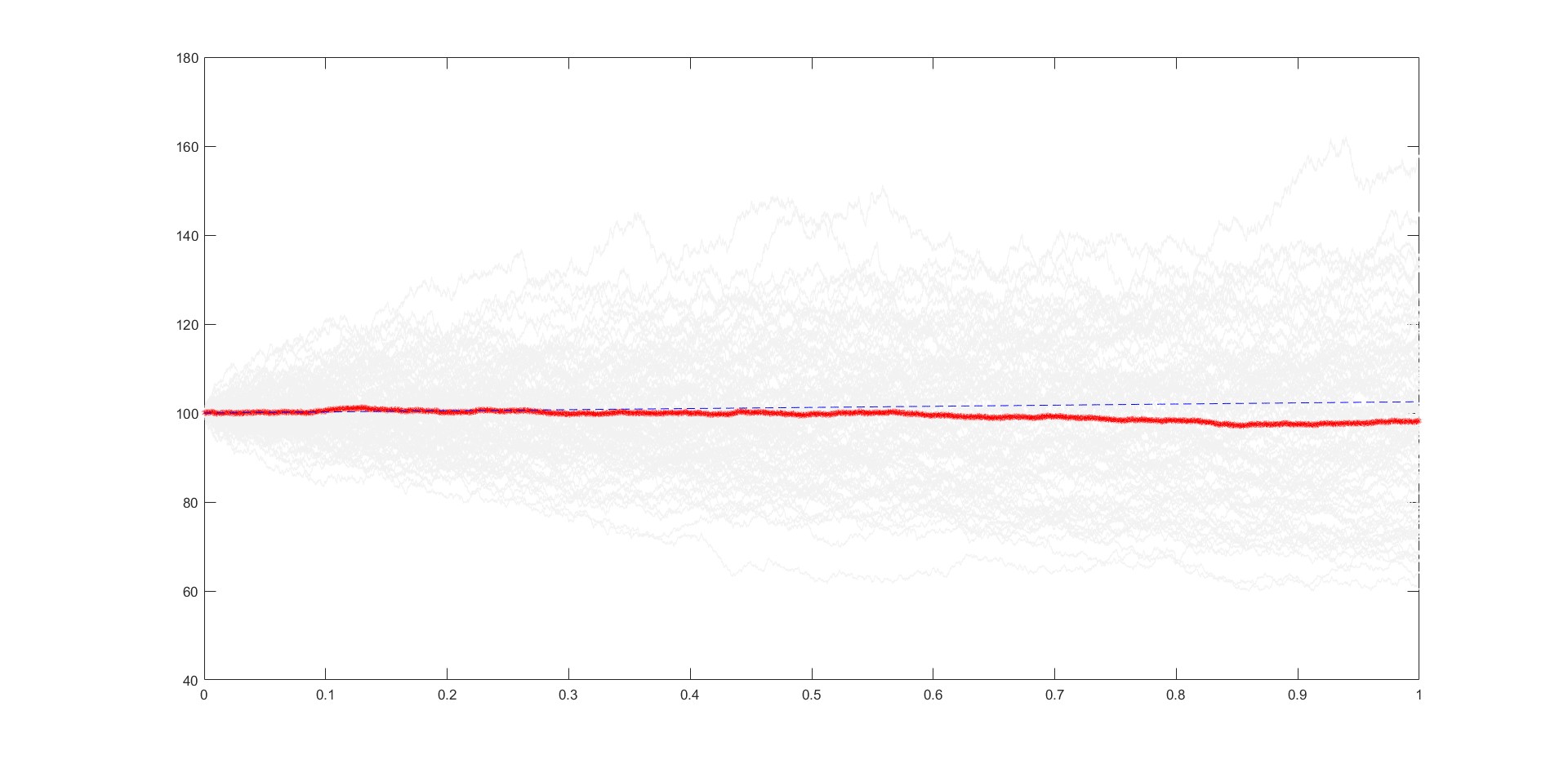
It would be rather useful to check whether our previous work is correct by comparing it with something that is certainly correct. We shall do this by comparing the result of our formulas with the result of a Monte Carlo estimation. Our simulation will be done using MATLAB. Consider an hypotethical asset-market combination with the following properties: \(S_{0}=100 \$\), \(r=2.5 \%\), \(\sigma = 20\%\). We will try pricing a down-and-out regular call with \(H=95\), \(T=1\) and \(K=102.5 \$\). It is essentially an ATMF call option with a knock-out clause. We will simulate 30000 paths: unfortunately Monte Carlo methods are slow to converge. Let’s take a look at the MATLAB code:

          % Pricing parameters
          mu = 0.025;
          sigma = 0.2;
          s_0 = 100;
          deltaTime=1/(252*8*12);
          numDataPoints=252*8*12;
          numPaths=30000;
          K=102.5;
          H=95;
          alpha=1-2*(mu/(sigma^2));

          % Asset paths simulation
          asset = gbm(mu,sigma,'StartState',s_0);
          tic;
          [X, T] = asset.simByEuler(numDataPOints, 'DeltaTime', deltaTime, 'nTrials', numPaths);
          toc
          assetPaths=zeros(numDataPoints+1,numPaths);
          for i=1:numPaths
                        assetPaths(:,i)=X(:,:,i);
          end

          % Option price estimation
          optionSimulatedPayoffs=zeros(1,numPaths);
          for k=1:numPaths
                        if min(assetPaths(:,k))<=H
                                      optionSimulatedPayoffs(k)=0;
                        else
                                      optionSimulatedPayoffs=max(assetPaths(end,k)-K, 0);
                        end
          end

          optionEstimatedPrice=exp(-mu)*mean(optionSimulatedPayoffs);
          optionExactPrice=blsprice(s_0,K,mu,1,sigma) - ((s_0/H)^alpha).*blsprice(H^2/s_0,K,mu,1,sigma);

The code is very much self explainatory, and for details about stochastic processes simulation one should refer to the official documentation by MathWorks. One might wonder why the number of data points is such that we are considering observations taken every quarter of an hour over a day (or taken every five minutes over an 8-hours working day). If we were to consider observations taken at the end of each trading day, we would be giving an overly optimistic and biased estimate of the option price as we would be discarding effects due to intraday volatility. To make a long story short, our asset may breach the barrier in between observation points, and we wouldn’t be able to notice that. Our estimated price is \(V=4.39(8)\$\). Assuming an approximately normal distribution for the estimator (can you spot any issues with this?) we get a standard error of \(0.06(8) \$\) and our theoretical price of \(4.34(5) \$\) is within the 95% confidence interval of our estimation. We can conclude that our Monte-Carlo estimate and our closed-form analytical formula agree on the result to a sufficient degree that we can confidently assign a price to the option.

Static hedging of barrier options

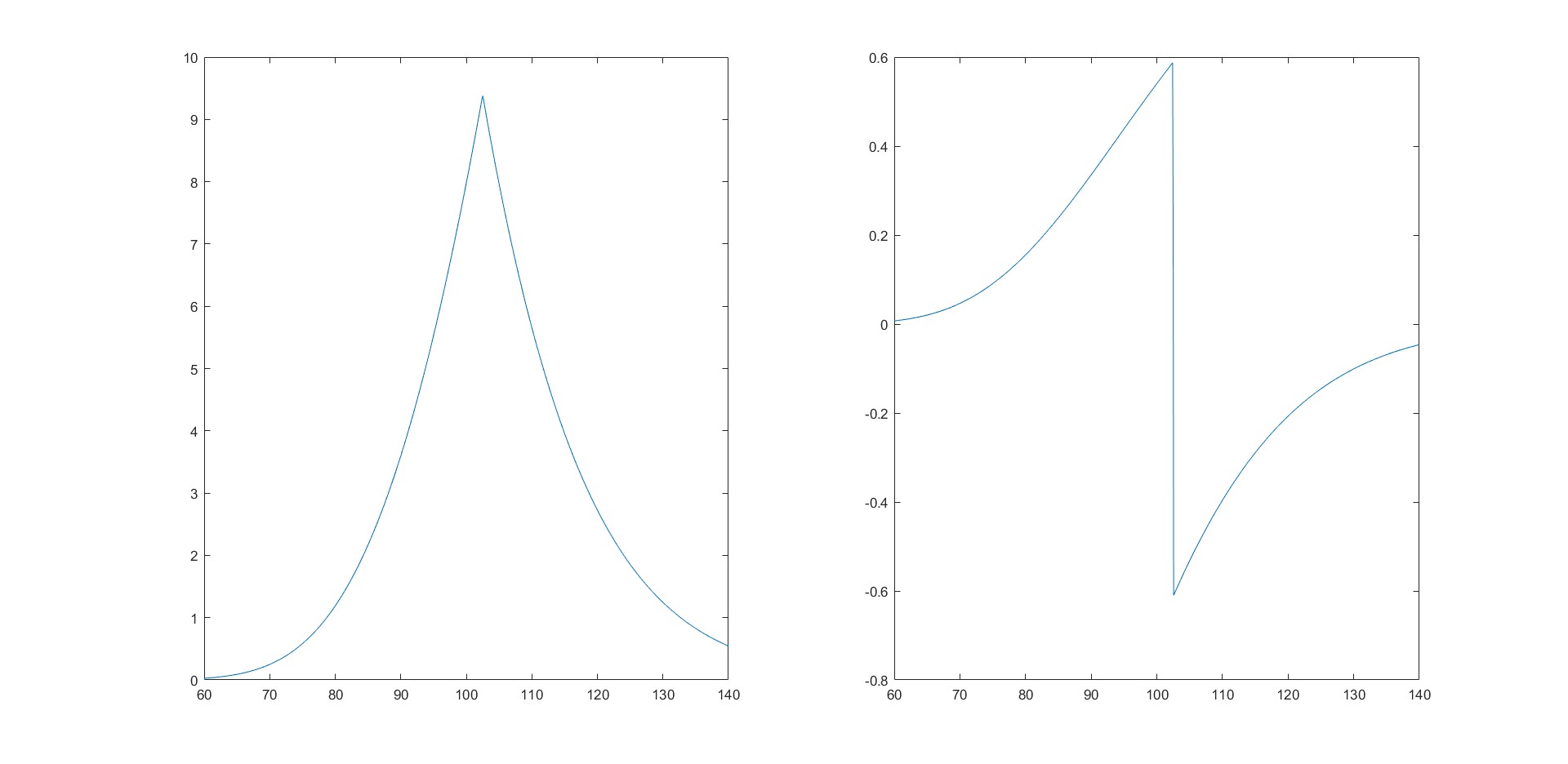
Once the appropriate formula for a price is found, it is natural to ask ourselves how to hedge a position involving barrier options. Unfortunately, when taking derivatives to evaluate \(\Delta\), the indicator functions induce finite jump discontinuities in the result. This means that hedging a position when the underlying is near the barrier can be extremely problematic, and static hedging techniques are out of the scope of this article. In the last 20 years the literature about solving this issue has been very abundant, so a search on Google Scholar can be a good starting point for learning more.

Getting creative: pricing a floating strike lookback call

At the heart of our work lies the issue of path-dependency. That is, our contract function is not only a function of information known at the time of expiration, but it also depends on other times preceding the expiration. Our clever solution with reflections had the only goal of removing path-dependency from our calculations. Now we will take a look at another contract that exhibits path dependency. Floating strike lookback calls are options that allow us to buy an asset at the lowest price recorded in between issuance of the option and expiration. Our contract function looks like this:

\begin{equation} \Phi = S_{T} - \min_{t= \tau} S_{\tau} \end{equation}

We will obtain a pricing formula decomposing this contract in a portfolio of options that are either not path-dependent or whose path-dependency we can manage. Let \(t\) be some time before expiration. Let \(\tau(t)\) be the time where our asset reached it lowest price, that is let \(\tau(t) = \arg \min _{t} S_{t}\). Intuitively, our portfolio must start with a plain vanilla call option, struck at \(S_{\tau(t)}\), given that surely we’ll have the right to buy the asset at such price. Then, our portfolio must take into account the possibility that the asset will fall even lower than \(S_{\tau(t)}\). We will add something to our portfolio that satisfies the following requirements:

• we must be able to price it using reflections;
• no benefit must be provided at expiration if \(S_{\tau(t)} = S_{\tau(T)}\);
• the resulting portfolio must be a call struck at \(S_{\tau(T)}\) (i.e. our lookback option).

We claim that this result can be achieved by adding infinitely many contracts, each one of them being bought in infinitesimal quantity. Consider for any \(\gamma\) lesser than \(S_{\tau(t)}\), a position obtained by going short \(d\gamma\) units of a down-and-in digital call struck at \(S_{\tau(t)}\) with barrier at \(\gamma\) and going long by the same amount on a down and in digital call struck at \(\gamma\) with barrier at \(\gamma\). Let’s check our claim:

• we can price digital DICs using reflections;
• since any \(\gamma\) is lesser than \(S_{\tau(t)}\), if \(S_{\tau(t)} = S_{\tau(T)}\) none of our contracts are active, and the payoff is null.
• suppose that \(S_{T}\) is greater than \(S_{\tau(t)}\). Integrate the payoff over the active, non zero value contract region (i.e. between \(S_{\tau(t)}\) and \(S_{\tau(T)}\)): \(\int_{S_{\tau(T)}}^{S_{\tau(t)}} d\gamma = S_{\tau(t)} - S_{\tau(T)}\). Then add to our previous result the payoff of our plain vanilla call: it is \(S_{T}-S_{\tau(t)}\), and therefore we obtain the right quantity. If \(S_{T}\) is lesser than \(S_{\tau(t)}\), the above integral reduces to \(\int_{S_{\tau(T)}}^{S_{T}} d\gamma = S_{T} - S_{\tau(T)}\), and adding the null payoff of the plain vanilla call yields again the correct result.

All of this allows us to state that the the price for a lookback floating strike call is given by

\begin{equation} \int_0^{S_{\tau(t)}} \left( C^{DIC,digital}(S_{t}, t, \sigma, r, \gamma, \gamma) - C^{DIC,digital}(S_{t}, t, \sigma, r, \gamma, S_{\tau(t)} \right) d\gamma + C^{call}(S_{t}, t, \sigma, r, S_{\tau(t)}) \end{equation}

You’ll be delighted to know that this integral allows for a closed form analytical solution, but solving the integral requires a certain bravery, a bit of time and a ton of paper. If you’re up for a nice integration challenge, go for it. You will find out that the solution is

\begin{equation} S_{t}e^{-r(T-t)}N(d_{1})-S_{\tau(t)}e^{-r(T-t)}N(d_{2})+S_{t}e^{-r(T-t)} \sigma \sqrt{T-t} \left[ \frac{1}{\sqrt{2\pi}} e^{- \frac{d_{1}^2}{2}}+d_{1}N(-d_{1}) \right] \end{equation}

where \(N(x)\) is the standard gaussian cdf. and \(d_{1}\) and \(d_{2}\) are the usual Black-Scholes quantiles evaluated for \(K=S_{\tau(t)}\) and \(S=S_{t}\). This expression is somewhat more complex if we allow for the presence of dividends, but the reasoning remains the same. Again feel free to try, I’m sure you’ll manage as it’s mostly a matter of making the right choices while integrating by parts.

Conclusions

We have seen how the reflection principle allows us to get rid of path-dependency and lets us find pricing formula that would be otherwise much more tedious to evaluate. This is not the only way possible: you may want to look into the theory of absorbed processes. This is the way that these formula were first found (see Muisela and Björk), and it is a perfecty valid one, although much more mathematically intense. The beauty of the reflection principle lies in the possibilty of being able to reason in financial terms, and the math just gets out of the way. This article is a good starting point, but much more can be said about path-dependent contract functions. Some possible next steps from here:

• looking into more contracts, such as ladders and double barriers;
• looking at how things change when we have stochastic dividends and rates;
• looking at the classic heat diffusion model (interestingly, the option pricing problem is very similar to the problem of predicting temperature evolution across an infinitely long rod), and then looking at the heat diffusion model with constant temperature zones (you will find that they behave very much like our barriers).

This is my first article for this blog, and my first attempt at blogging in general. Reach out to me on Linkedin or GitHub if you want to suggest improvements or if you want to just have a chat about this. I hope that you enjoyed!

Bibliography and further reading

• Pricing options under the Vasicek model
• Static hedging of barrier options
• Björk, Tomas, 2009. “Arbitrage Theory in Continuous Time”. Professor Björk passed away in 2021: although I never met him, I am still very grateful for this work of his from which I learned the fundamentals of finance in continuous time. A must-read for all who aspire to work in this field.
• Effects of intraday volatility on Monte Carlo estimates.
• Musiela, Mark & Rutkowski, Marek, 2004. “Martingale Methods in Financial Modelling”.

Updates

• 12/10/2022 - Rolled back to MathJax version 2.7 to improve mobile-friendliness: TeX sections have been modified accordingly. Fixed some typos.